GELU: Gaussian Error Linear Units

Date: July 22, 2024

Estimated Reading Time: 20 min

Author: Hector Motsepe

Activation functions are crucial components in neural networks, introducing non-linearity and enabling the network to learn complex patterns. From a mathematical standpoint, an activation function f(x) is a non-linear transformation applied to the output of a neuron:

y = f(Σ(w_i * x_i) + b)

Where:- x_i are inputs - w_i are weights - b is a bias term - Σ denotes summation

Without activation functions, neural networks would be limited to learning linear transformations. The composition of linear functions is still linear:

f(g(x)) = (ax + b)(cx + d) = acx^2 + (ad + bc)x + bd

This is still a linear function in terms of its parameters, limiting the network’s expressivity. Non-linear activation functions allow the network to approximate any function, as per the Universal Approximation Theorem. Let’s look at the historical transformation of activation functions to build the motivation behind GELU.

A Brief History

1. Sigmoid Function

σ(x) = 1 / (1 + e^(-x))

One of the earliest activation functions, the sigmoid squishes the input values into a range between 0 and 1. While it introduced non-linearity and had a clear probabilistic interpretation, it still suffered from the vanishing gradient problem in deep networks.
The vanishing gradient problem occurs when the gradients of the loss function approach zero therefore making the network harder to train. As abs(x) increases, σ’(x) approaches 0, leading to vanishing gradients during backpropagation.

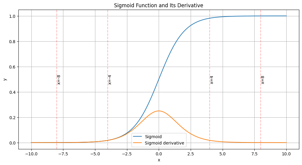
Fig 1: Sigmoid Function and Its Derivative

The above graph indicates that the derivative (gradients) of the sigmoid function approaches zero as the absolute value of x increases.

2. Tanh Function

tanh(x) = (e^x - e^(-x)) / (e^x + e^(-x))

While tanh offers a broader output range (-1 to 1), it still suffers from vanishing gradients for large inputs. As abs(x) increases, tanh’(x) also approaches 0:

tanh'(x) = 1 - tanh^2(x)

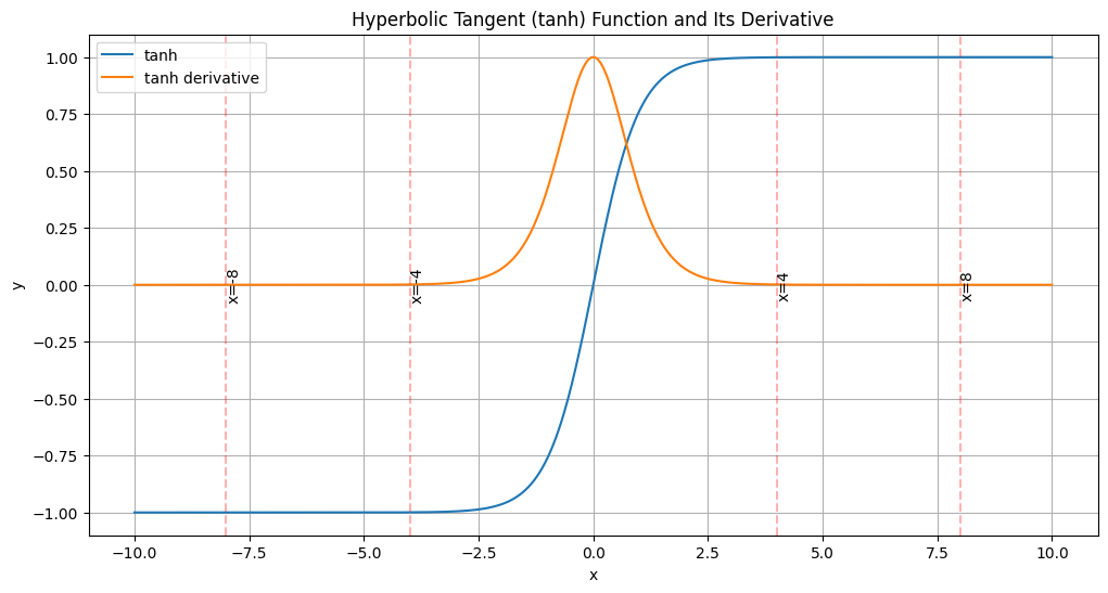
Fig 2: Tanh Function and Its Derivative

3. ReLU

ReLU(x) = max(0, x)

Both sigmoid and tanh compress an infinite input range into a finite output range. This compression leads to information loss, especially for inputs with large magnitudes.

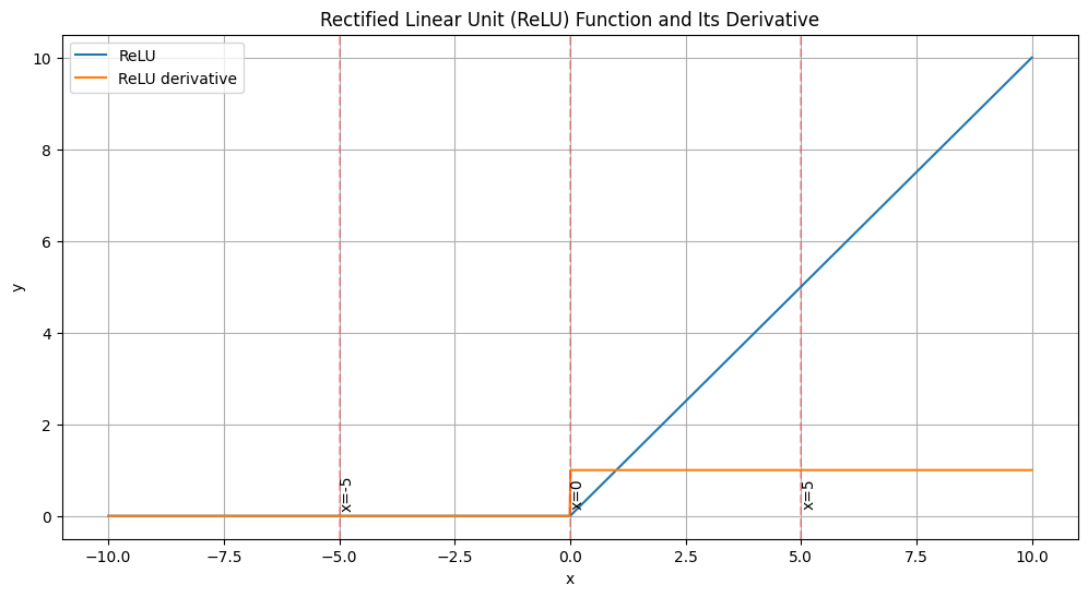
Fig 3: ReLU Function and Its Derivative

ReLU gradient is 1 for all the positive inputs (x > 0), which helps mitigate the vanishing problem. At x = 0, the derivative is undefined (usually set to 0 or 1 in practice). However, ReLU introduces its own challenge: the “dying ReLU” problem, where neurons can become permanently inactive for all inputs. If a neuron’s weights are updated such that it always receives negative inputs, it will never activate and never update (it dies).

GELU: Bridging Deterministic and Stochastic Approaches

Gaussian Error Linear Unit (GeLU) is one of the most used activation functions in deep learning. The activation function was used in GPT-3 (Brown et al., 2020), and BERT (Devlin et al., 2018).

The GeLU offers a novel approach:

GELU(x) = x * Φ(x)

Where Φ(x) is the Cumulative Distribution Function (CDF) of the standard normal distribution. The Normal (or Gaussian) distribution is a probability distribution that appears frequently in nature and is central to many statistical methods. It’s characterized by its bell-shaped curve and is defined by two parameters: the mean (μ) and standard deviation (σ). The author chooses the standard normal distribution because the neuron inputs tend to follow a normal distribution. Batch Norm, Central Limit Theorem, and Weight Init strategies support this assumption.

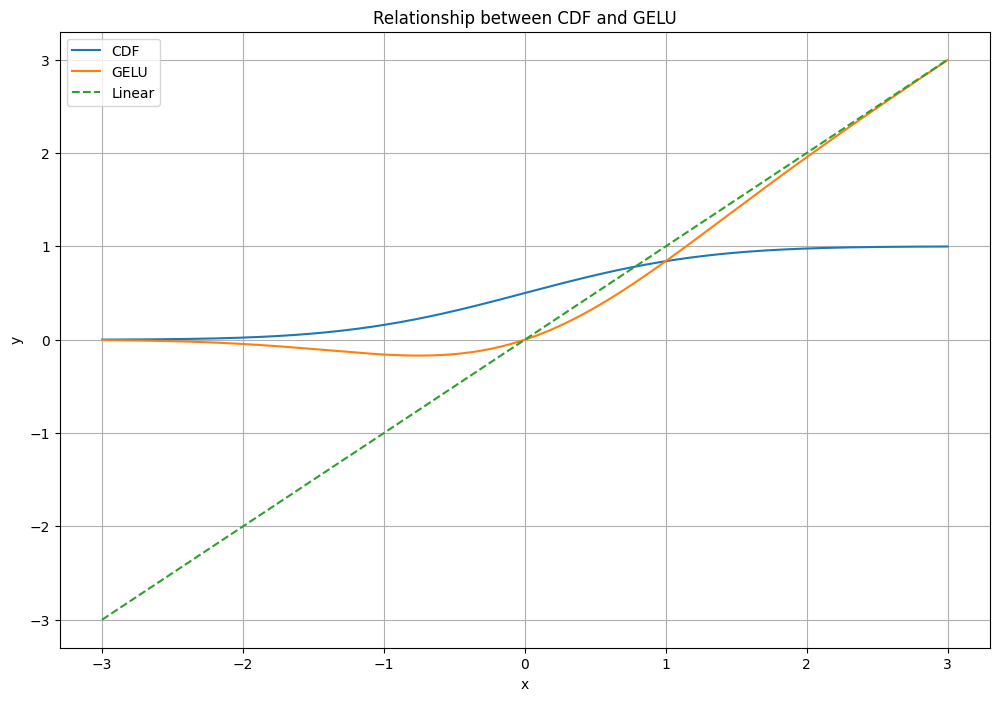
Fig 4: Cumulative Distribution Function

The CDF of a probability distribution F(x) gives the probability that a random variable X takes on a value less than or equal to x: F(x) = P(X ≤ x). For example: For x = 0, Φ(0) ≈ 0.5 (there’s a 50% chance of picking a number less than or equal to 0). As x increases, Φ(x) approaches 1 (it becomes more likely to pick a number less than x). As x decreases, Φ(x) approaches 0 (it becomes less likely to pick a number less than x).

Since the cumulative distribution function of a Gaussian is often computed with the error function, the author defines the Gaussian Error Linear Unit (GELU) as:
\(\text{GELU}(x) = x P(X \leq x) = x \Phi(x) = x \cdot \frac{1}{2}\left[1 + \text{erf}(x/\sqrt{2})\right]\)

GELU combines properties from Dropout, zoneout, and ReLUs potentially offering:

Deterministic Property:

ReLU is a deterministic activation function because for any given input, it always produces the same output:

ReLU(x) = max(x, 0); ReLU'(x) = {1 if x > 0, 0 otherwise}

Stochastic: Dropout

Dropout, while not an activation function per se, introduces stochasticity (randomness) into the network:

y = f(Σ(w_i * x_i * z_i) + b)

Where z_i ~ Bernoulli(p), i.e., z_i is 1 with probability p and 0 with probability 1-p. During training, this randomly “drops out” neurons, creating an ensemble effect. At inference time, this is typically approximated by scaling the weights by p.

GeLU: Merge both deterministic and stochastic properties

GeLU multiplies the input by zero or one, but these values are stochastically determined while being dependent on the input. For instance, the neuron input x is multiplied by m ∼ Bernoulli(Φ(x)), where Φ(x) = P(X ≤ x), X ∼ N (0, 1) is the cumulative distribution function of the standard normal distribution (Hendrycks et al., 2016).

Mitigation of vanishing gradients, smooth, differentiable behavior

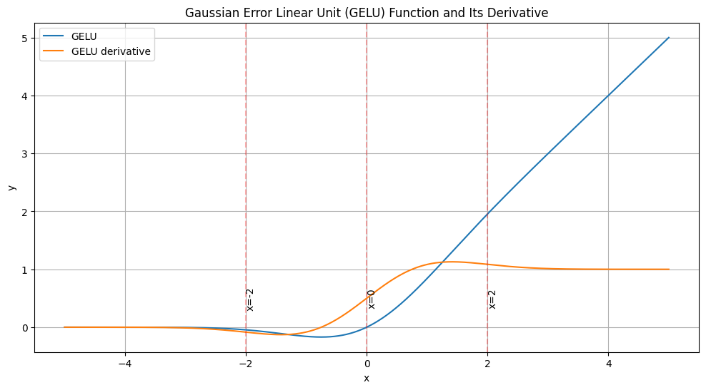
Fig 5: Smooth GeLU

As indicated in the above graph, GeLU offers a smoother transition as it greatly curves upward for positive inputs and softly approaches zero for negative inputs without sudden jumps or kinks. ReLU, on the other hand, is characterized by the sharp bend at x=0. This smoothness of GELU has significant implications for gradient flow during backpropagation. In ReLU, the gradient is either 0 (for negative inputs) or 1 (for positive inputs), with an undefined point at exactly x=0. This binary nature can cause problems, particularly the “dying ReLU” phenomenon, where neurons get stuck in a state where they always output zero, effectively becoming useless.
GELU sidesteps this issue elegantly. Its derivative is smooth and continuous everywhere, providing a non-zero gradient even for slightly negative inputs. This means that neurons using GELU are less likely to “die” compared to those using ReLU. Even if a neuron receives predominantly negative inputs, there’s still a chance for it to recover and contribute meaningfully to the network’s computations.

Summary

This blog explored:

1. The Evolution of Activation Functions:
   • From sigmoid and tanh to ReLU, highlighting their strengths and limitations.
   • The persistent challenge of vanishing gradients in deep networks.
2. GELU’s Unique Approach:
   • Combines deterministic and stochastic properties.
   • Utilizes the cumulative distribution function of the standard normal distribution.
3. Key Advantages of GELU:
   • Smooth, differentiable behavior that mitigates vanishing gradients.
   • Reduces the “dying neuron” problem associated with ReLU.
   • Offers a balance between deterministic activation (like ReLU) and stochastic regularization (like Dropout).
4. Mathematical Foundations:
   • Explores the underlying principles and formulas that define GELU.
   • Discusses how GELU relates to probability theory and statistical concepts.

References

• Brown, T. B., Mann, B., Ryder, N., Subbiah, M., Kaplan, J., Dhariwal, P., … & Amodei, D. (2020). Language models are few-shot learners. arXiv preprint arXiv:2005.14165.
• Devlin, J., Chang, M. W., Lee, K., & Toutanova, K. (2018). BERT: Pre-training of deep bidirectional transformers for language understanding. arXiv preprint arXiv:1810.04805.
• Hendrycks, D., & Gimpel, K. (2016). Gaussian Error Linear Units (GELUs). arXiv preprint arXiv:1606.08415.