Evaluating Learning Rate Scheduling Techniques on Mr. Karpathy’s GPT-2

Recently, Mr. Andrej Karpathy trained GPT-2 from scratch using the Cosine Schedule learning rate. Inspired by this, I decided to test various learning rate scheduling techniques to see how they improve the performance, convergence speed, and training stability of AK’s GPT-2 model. Before we get into the experimentation, lets build the intuition first.

Understanding Learning Rates

• Definition: Learning rates determine the step size in an optimization algorithm at each iteration, guiding the movement towards the minimum of a loss function (Murphy, 2012).
• Importance: Learning rates influence how newly acquired information overrides old information, affecting how the model “learns.”
• Function: The gradient of the loss determines the descent direction, while the learning rate determines the step size in that direction.

Setting the Learning Rate

• Trade-offs: Balancing between the rate of convergence and overshooting is crucial.
  • High Learning Rate: Can cause the learning to jump over minima.
  • Low Learning Rate: Can lead to slow convergence or getting stuck in undesirable local minima.
• Adaptation: Finding a sweet spot or adapting the learning rate during training is essential.

Techniques

• Decay-Based Learning Rate: Gradually reducing the learning rate over time allows the model to make larger updates initially and smaller updates as training progresses, avoiding overshooting around the optimum.
• Step/Time-Based Learning Rate: Altering the learning rate based on previous iterations.

Experimentation

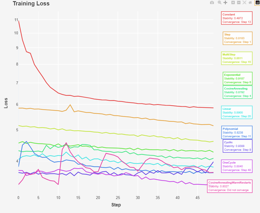
Fig 1: Training Loss over Training Step For different types of Learning rate Scheduler

The above graph indicates that the training loss over training step for different learning rate schedulers. We see that ConstantLR lead to slow convergence, and doesn’t reach the lowest loss as it doesnt adapt to the changing curvature of the loss landscape. As shown in the below code the learning rate stay constant across the entire training loop.

@dataclass
class ConstantLR:
    max_lr: float = 3e-4

    def __call__(self, iteration: int) -> float:
        return self.max_lr

The StepLR start with a high learning rate and then reduce it at each itercation, therfore allowing for finer adjustements and faster intial progress. The StepLR reduces the learning rate by a decay factor “gamma”. Think of it as gamma determinming our decay rate at each iteration. Based on the above grpah the learning rate reaches Final Loss of 5.151307. As shown below gamma is a hyperameter, we need to manually determine how we should decay our learning rate this can affect our convergence speed.

@dataclass
class StepLR:
    max_lr: float = 6e-4
    max_iters: int = 50
    gamma: float = 0.95

    def __call__(self, iteration: int) -> float:
        return self.max_lr * (self.gamma ** (iteration // self.max_iters))

The MultiStepLR starts with higher learning rate and then reduce it after reaching specific step “milestones”. Unlike StepLR the learning can stay unchanged until reaching the next milstones. Gamma is “decay factor” is a hyperparameter requires manual tuning.

@dataclass
class MultiStepLR:
    max_lr: float = 6e-4
    max_iters: int = 50
    gamma: float = 0.95
    milestones: List[int] = (15, 30, 45)

    def __call__(self, iteration: int) -> float:
        return self.max_lr * (self.gamma ** sum([iteration >= m for m in self.milestones]))

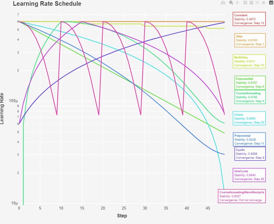
Fig 2: Learning Rate Schedules

The LinearLR decreases linearly from the initial learning rate (self.max_lr) to zero over the course of the training. It starts at self.max_lr (the maximum learning rate) As iteration increases, the learning rate decreases linearly. When iteration reaches self.max_iters, the learning rate becomes 0. The learning rate reached the Final Loss of 3.830209. I think the reason it is better than MultiStep and StepLR is because the iteraction determine the rate of decay and not gamma.

@dataclass
class LinearLR:
    max_lr: float = 6e-4
    max_iters: int = 50

    def __call__(self, iteration: int) -> float:
        return self.max_lr * (1 - iteration / self.max_iters)

The ExponentialLR The learning rate decreases exponentially with each iteration. This means that the learning rate will drop rapidly at the beginning of the training and more slowly as training progresses. Exponential decay is often used to quickly reduce the learning rate early in training and then slow down the rate of decay as the model approaches convergence. The Final Loss: 4.263788 and had the best training stability score: 0.9187

@dataclass
class ExponentialScheduler:
    max_lr: float = 6e-4
    gamma: float = 0.95

    def __call__(self, iteration: int) -> float:
        return self.max_lr * (self.gamma ** iteration)

The CosineScheduler is one of the mostly used learning rate schedule. The learning rate starts from a minimum value and increases linearly during the warmup phase (0 to max_lr). After the warmup phase, the learning rate follows a cosine decay schedule from a maximum value to a minimum value (max_lr to min_lr) over a specified number of iterations. Cosine Annealing had a stable training run 0.87 and final loss of 4.081490

 @dataclass
class CosineScheduler:
    max_lr: float = 6e-4
    min_lr: float = 3e-5 # AK max_lr * 0.1
    warmup_iters: int = 1000
    max_iters: int = 50

    def __call__(self, iteration: int) -> float:
        if iteration < self.warmup_iters:
            return self.max_lr * iteration / self.warmup_iters

        if iteration > self.max_iters:
            return self.min_lr

        decay_ratio = (iteration - self.warmup_iters) / (self.max_iters - self.warmup_iters)
        assert 0 <= decay_ratio <= 1

        coeff = 0.5 * (1.0 + math.cos(math.pi * decay_ratio))
        return self.min_lr + coeff * (self.max_lr - self.min_lr)

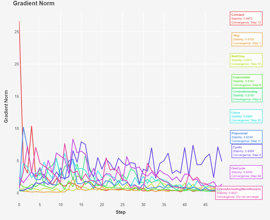
Fig 3: Gradient Norm

The PolynomialLR The learning rate starts from a maximum value and decays to a minimum value over a specified number of iterations, following a polynomial function. The power parameter is the power of the polynomial, which controls the rate of decay. This type of decay allows for more flexible control over the learning rate schedule compared to linear decay. By adjusting the power parameter, you can control how quickly the learning rate decreases

• power < 1: The learning rate will decay more slowly at the start and more quickly towards the end (convex curve).
• power = 1: The learning rate decays linearly (straight line).
• power > 1: The learning rate will decay more quickly at the start and more slowly towards the end (concave curve).

@dataclass
class PolynomialLR:
    max_lr: float = 6e-4
    min_lr: float = 3e-5 # AK max_lr * 0.1
    max_iters: int = 50
    power: float = 2.0

    def __call__(self, iteration: int) -> float:

      # Fraction of Iterations Completed * Fraction of Iterations Remaining ** Polynomial Decay + Shift by min_lr (Ensures the learning rate never falls below min_lr)
        return (self.max_lr - self.min_lr) * (1 - iteration / self.max_iters) ** self.power + self.min_lr

The OneCycleLR is a variation of the cyclic learning rate that includes a single cycle with a warmup and cooldown period. Almost similar to Annealine Cosine, This scheduler starts with a low learning rate, increases it to a maximum, and then decreases it again. This approach can help the model quickly converge to a good solution while maintaining stability. had the best training stability of 0.9388 and the lowest loss; Final Loss: 3.355333

The policy is designed to maximize performance by first rapidly increasing the learning rate to explore the loss landscape and then gradually decreasing it to fine-tune the model.

@dataclass
class OneCycleLR:
    max_lr: float = 6e-4
    min_lr: float = 3e-5
    max_iters: int =  50
    pct_start: float = 0.3 #  The fraction of max_iters during which the learning rate increases from min_lr to max_lr.

    def __call__(self, iteration: int) -> float:
        if iteration / self.max_iters <= self.pct_start:
            return self.min_lr + (self.max_lr - self.min_lr) * (iteration / (self.pct_start * self.max_iters))
        else:
            return self.max_lr - (self.max_lr - self.min_lr) * ((iteration - self.pct_start * self.max_iters) / ((1 - self.pct_start) * self.max_iters))

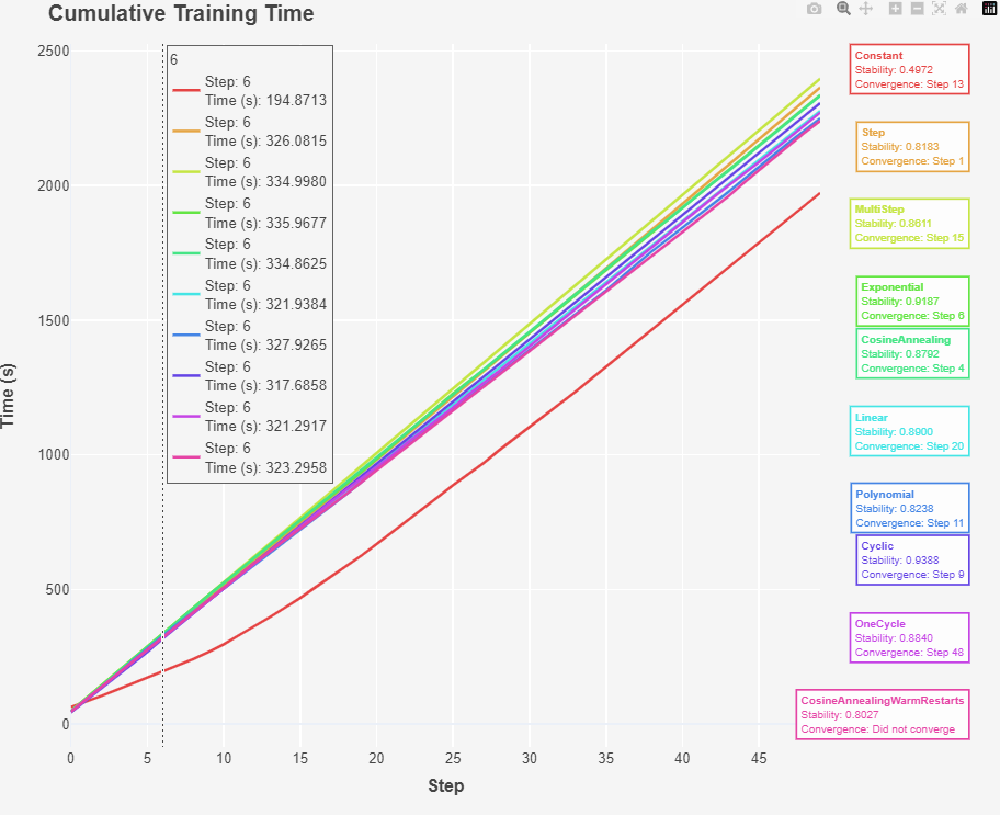
Fig 4: Training time

The CosineAnnealingWarmRestarts: Ther Fastest scheduler: CosineAnnealingWarmRestarts (2240.12 seconds) and Slowest scheduler was MultiStep (2397.08 seconds). This CosineAnnealingWarmRestarts scheduler combines the benefits of cosine annealing with periodic resets, potentially allowing the model to escape local minima and explore different regions of the loss landscape.

• Warm Restarts: Periodically resetting the learning rate to a higher value can help the model escape local minima and continue improving. However, this can cause spikes in the norm and loss as shown in Fig 1 and 3. The training stability of was 0.80

@dataclass
class CosineAnnealingWarmRestarts:
    max_lr: float = 6e-4
    min_lr: float = 3e-5
    warmup_steps: int = 10
    T_mult: int = 1

    def __call__(self, iteration: int) -> float:
        T_cur = iteration % self.warmup_steps
        T_i = self.warmup_steps
        while iteration >= T_i:
            iteration -= T_i
            T_i *= self.T_mult
        return self.min_lr + (self.max_lr - self.min_lr) * (1 + math.cos(math.pi * T_cur / self.warmup_steps)) / 2

The CyclicLR: The cyclic nature of this schedule allows the learning rate to oscillate between a minimum and maximum value. This can help the model explore a broader range of learning rates and avoid getting stuck in local minima.

@dataclass
class CyclicLR:
    max_lr: float = 6e-4
    min_lr: float = 3e-5
    max_iters: int = 50

    def __call__(self, iteration: int) -> float:
        # we determines which full cycle the current iteration is in.
        cycle = math.floor(1 + iteration / (2 * self.max_iters))
        # then Normalizes the iteration position within the current cycle.
        x = abs(iteration / self.max_iters - 2 * cycle + 1)  
              # scale
        return self.min_lr + (self.max_lr - self.min_lr) * max(0, (1 - x))

References

• Murphy, Kevin P. (2012). Machine Learning: A Probabilistic Perspective. Cambridge: MIT Press. p. 247. ISBN 978-0-262-01802-9.

- Code for Reproducibility can be found here: https://github.com/Motsepe-Jr/gpt2